Visualization of the Seismic Wave Propagation
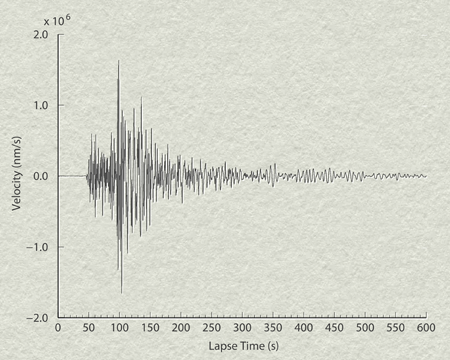
1D. f = f(t)
This is the standard way to describe the seismic wave, called "seismogram". We can see the shaking at a particular place.
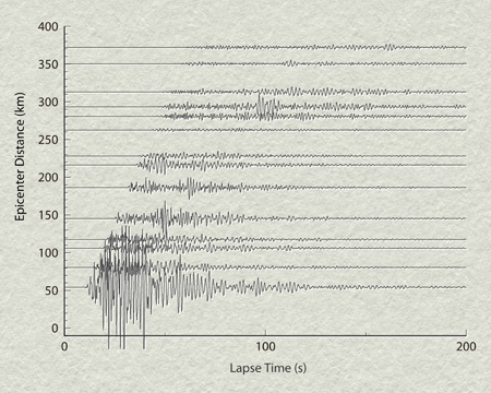
2D. f = f(x, t)
We can see the propagation of the seismic wave, for example, the P and S wave propagation. We need multiple stations to make this figure.
3D. f = f(x, y; t). 2D space + time
The seismic wave energy is plotted at each station at a particular time in 2D map. We can convert a lot of maps with different lapse times into a movie. By making the movie, we can see introduce one additional dimension.
3D. f = f(x, y; t). 3D expression of 2D data + time
By showing the energy as a height field, we can make 3D image. This movie is more impressive than the previous one.
4D. f = f(x, y, f; t). 3D data + time
This movie shows the seismic energy of different frequencies. The vertical direction means the frequency: the surface and the top most correspond to 0.1Hz and 05Hz, respectively. We can see aftershocks having high frequency component.
4D. f = f(x, y, z; t). 3D data + time
At each station, UD, NS and EW components are recorded. We can calculate the particle motion by using three components. In this movie, we can see the shaking motion of the Rayleigh wave. By using the Google Earth, we can change the view point as we want.
Acknowledgement
All of the data used in this page is downloaded from the web site of Hi-net managed by NIED.